Does
Oracle have a Sense of Humour?
by Jaromir
D.B. Nemec
Among all
DBMS evaluations I encountered there were a lot of features checked
(functionality, licence policy, support, to name a few), non of those features was
the sense of humour. It's a pity! I’m sure that at least some of the database
management systems posses this ability. Read this true story.
Cross with Table T
Consider an
ordinary fact table in an average data warehouse environment; let’s call our table
“T”. Like all fact tables table T posses several dimensions keys (more
precisely said, the table T contains foreign keys of the associated dimension
tables).
Lets call
one of those dimensions “D”, the foreign key defined in the table T is D_ID.
One of the
most elementary tasks is to select all
rows from the fact table T associated with particular keys of the dimension D.
SQL> select * from
t where d_id in (1111,1112,1113,1114,1115);
. . . . .
9 rows selected.
Elapsed: 00:00:55.31
Execution Plan
--------------------------------------------------------------------------
| Id | Operation | Name | Rows |
Bytes | Cost (%CPU)| Time |
--------------------------------------------------------------------------
| 0 | SELECT STATEMENT |
| 49025 | 5601K| 16053 (1)| 00:02:41 |
|* 1 |
TABLE ACCESS FULL| T | 49025
| 5601K| 16053 (1)| 00:02:41 |
--------------------------------------------------------------------------
Well this
is not really the response time an average user would be satisfied with. What’s
wrong here? Our dimension D is somehow skew.
The wrong guess (cardinality 50K instead of 9 rows) leads to a full scan
of the table.
This
dimension is a typical dimension positioned somewhere between the
identification dimensions (uniquely identifying each entity) and say category
dimensions (with relatively low cardinality). The dimension D has following
properties:
- there are (few) dimension keys
with lot of records in the fact table (most popular products)
- there are (many) dimension keys
with very few records in the fact table (exotic, highly customised
products)
- the total number of dimension
keys is higher then 254 (we will see the meaning of this “magical number”
in a while).
The table T
has 10M rows. The DDL for the table are shown below.
create table t
(d_id number,
x_id number,
y number,
pad char(100));
create index t_idx on t(d_id);
create index t_idx2 on t(x_id,y,d_id);
The script
populating the table with sample data is shown below.
Let’s Use a Hint
The problem
is very straightforward. We know the predicate would return only a few numbers
of records from the table T (for example 9 rows as we saw above) , but the
optimiser doesn’t know that. It assumes that the result cardinality will be
much higher and prefers to use full table scan over an index range scan access
(repeated for all members of the IN list).
Well, what
about to hint the optimiser to use the index defined on the dimension key?
Nothing easier, the INDEX() hint is
here exactly for this purpose.
SQL> select /*+
INDEX(t) */ * from t where d_id in (1111,1112,1113,1114,1115);
. . . .
9 rows selected.
Elapsed: 00:00:00.23
Execution Plan
--------------------------------------------------------------------------------------
| Id | Operation | Name
| Rows | Bytes | Cost (%CPU)|
Time |
--------------------------------------------------------------------------------------
| 0 | SELECT STATEMENT | | 49025 | 5601K|
49144 (1)| 00:08:12 |
| 1 |
INLIST ITERATOR
| | |
| | |
| 2 |
TABLE ACCESS BY INDEX ROWID| T | 49025 | 5601K|
49144 (1)| 00:08:12 |
|* 3 |
INDEX RANGE SCAN | T_IDX
| 49025 | | 112
(0)| 00:00:02 |
--------------------------------------------------------------------------------------
Excellent;
consider the difference in response time as a result of using the T_IDX index
in iterated range scan. But wait a moment, actually there is no need to perform
the select star, the only column we need to select is the column x_id. Let’s
rewrite the select and start it again.
SQL> select /*+
INDEX(t) */ x_id from t where d_id in (1111,1112,1113,1114,1115)
;
. . . .
9 rows selected.
Elapsed: 00:00:21.67
An
interesting result; selecting less data results in worse elapsed time! We will
examine the execution plan in a while to see the difference.
The Joke
Let’s me
paraphrase the discussion between the user and the CBO as follows:
USER: I
have some very simple select:
select /*+ INDEX(t) */ x_id from t where d_id in (1001,1002,1003,1004,1005);
Please
perform it!
CBO: Hint
index?
USER: Sure!
I want to avoid the FTS.
CBO: OK, if
you insist …
---------------------------------------------------------------------------
| Id | Operation | Name | Rows | Bytes | Cost (%CPU)| Time |
---------------------------------------------------------------------------
| 0 | SELECT STATEMENT | | 49025 | 526K| 38125 (1)|
00:06:22 |
|* 1 |
INDEX FULL SCAN | T_IDX2 | 49025 |
526K| 38125 (1)| 00:06:22 |
---------------------------------------------------------------------------
USER: grrr
CBO: :)
Some Discussion
We used the
hint in the form INDEX(t), so any index on the table can be used. CBO examined
the second index T_IDX2 and found that the entire select could be performed
using only the index (not the table data). xxx
Ok, of
course we would omit the problem if we would specify the index exactly using
the full index hint syntax INDEX (table_name, index_name). As we can see, the
unqualified option of the INDEX hint
(“use index whatever you find appropriate”) is not always the best choice.
The second
point is, why doesn’t Oracle choose the index access on its own (i.e. without a
hint). Well, we mentioned this already,
the cardinality of the dimension is higher than 254.This forces the histogram
defined on the column D_ID to be height balanced. Compared with the frequency
histogram where the exact cardinality of each column value is stored, the
height balanced histogram itself is only an estimation of the reality. We
choose the sample data so that there is no popular value in the histogram (I
call this “stuffing out” of the histogram). This leads to the fact, that for
all values (for the very common ones as well as for the very rare ones) the estimated
cardinality is calculated as 1 / density.
The
comparison of the CBO estimation and reality is shown in Figure 1.
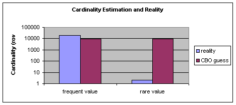
Figure 1 Cardinality estimation for the frequent and
rare column values
Finally
there is the question, why the CBO switches from the index range scan to the
index full scan? Well, the index full scan was preferred because of a similar
reason as in the initial query. The law of low costs rules!
The best
way to demonstrate this is to make a graph describing the dependency of the
cost on the cardinality of the IN list. We will consider three types of cost in
the graph:
- FTS (full table scan) – the
cost depends on the number of blocks of the table and the MBRC factor. The
cost is constant independent of the cardinality of the IN list.
- IFS (index full scan) - the
cost depends on the number of leaf blocks (and probably on the BLEVEL too,
but I ignore this). The cost is constant independent of the cardinality of
the IN list.
- IRS (index range scan) – the
cost depends on the number of leaf_blocks, clustering factor and the
effective index selectivity (equals to effective table selectivity in our
case). The cost is directly proportional to the cardinality of the IN
list.
Figure 2 gives
the answer; if the IN list consists of more that 3 members the index full scan
is preferred. If you don’t see this effect in your environment, you probably
have a different MBCR factor in your database (parameter
db_file_multiblock_read_count or system statistics) simply add some members to
the IN list.
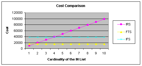
Figure 2 Cost Comparison for IRS (index range scan),
FTS (full table scan) and IFS (index full scan)
By the way,
why didn’t Oracle choose the index FAST full scan? Well, in this case this
would be perfectly meaningful, the access path using index fast full scan will
be much better than the single block read based index full scan. Apparently the
INDEX hint doesn’t trigger the index FAST full scan. This is OK; index FAST
full scan it not something one has usually in mind when hinting for INDEX!
The Script
This
behaviour was observed in Oracle 9i and reproduced in 10gR2 (with and without
the system statistics). The preference of full scans over index access is
particularly a behaviour of a data
warehouse database (e.g. with a relatively highly configured
dbfile_multi_block_read_count parameter.
create table t
(d_id number,
x_id number,
y number,
pad char(100));
--- stuff out histogram (with 255 different values)
insert into t
select
mod(rownum-1,255),
rownum, rownum,'x'
from dual
connect by level <= 5000000; --
--- and fill the table with approx. 1 records per dim. key
insert into t
select
1000+trunc(DBMS_RANDOM.VALUE(0,1)* 5000000),
rownum, rownum,'x'
from dual
connect by level <= 5000000;
--
commit;
--
create index t_idx on t(d_id);
create index t_idx2 on t(x_id,y,d_id);
--
begin
dbms_stats.gather_table_stats(ownname=>user, tabname=>'t',
method_opt=>'for all columns
size 254', cascade => true,
estimate_percent => 10);
end;
/
Some Useful Selects
While
investigating the table T there I found some select statement helpful.
Does the histogram contains popular values?
A popular
value can be identified on a gap in the
view user_tab_histogram as follows:
select a.*,
case when histogram =
'HEIGHT BALANCED' and
endpoint_number
-lag(endpoint_number,1,0)
over (order by endpoint_number) > 1 then 'popular
value' end popular_value
from user_tab_histograms a,
(select num_buckets,
num_distinct, histogram from user_tab_columns a
where table_name =
'T' and column_name like 'D_ID')
where table_name = 'T' and column_name
= 'D_ID'
order by table_name, column_name, ENDPOINT_NUMBER;
How is the DENSITY (in user_tab_columns) calculated?
According
to [OCBF] p.172, following algorithm is used (in case there is no popular value
in the histogram).
SQL> select sum(sq) / (sum(cnt) *
sum(cnt))
2 from (
3 select d_id,
count(*)*count(*) sq, count(*) cnt from t group by d_id
4 );
SUM(SQ)/(SUM(CNT)*SUM(CNT))
---------------------------
.000980492
This is
exactly what we see in the view USER_TAB_COLUMNS (note that you may get a
slightly different value, if you gather statistics with estimate_percent less
than 100). The value of num_rows * density (10,000,000 * .000980492
= 9805) is the
estimated cardinality for equation predicate. In case of IN list the predicate
is the cardinality multiplied with the number of members of the IN list.
How are the data for the
graph in Figure 2 calculated?
To
calculate the cost estimation, the appropriate formulae must be known, for the
full discussion see [OCBF]. Note that for the reason of simplicity, I omitted
some parts that have either marginal influence on the result or I assume they
have a marginal influence. Note, that the system statistics are considered to
be gathered.
select
inlist_cnt,
inlist_cnt *
(blevel +
ceil (leaf_blocks *
(select round(density,7)
from user_tab_columns
where table_name =
a.table_name
and column_name =
b.column_name)) +
ceil(clustering_factor *
(select round(density,7)
from user_tab_columns
where table_name = a.table_name
and column_name =
b.column_name))) cost_irs, -- cost
of index range scan [CBOF] p.69
(select
round(
((select blocks from dba_tables
where table_name = a.table_name) /
(select pval1 from
sys.aux_stats$ where pname = 'MBRC')) -- #MRds
*
(select pval1 from sys.aux_stats$ where pname = 'MREADTIM')/
(select pval1 from
sys.aux_stats$ where pname = 'SREADTIM') -- MRds correction
-- CPUcycles are ignored
) -- cost of full table scan
[CBOF] p.19
from dual) as cost_fts,
(select leaf_blocks from user_indexes where table_name = 'T' and index_name = 'T_IDX2')
-- ignored: CPU + BLEVEL processing
as cost_ifs -- cost of index fast full scan
from user_indexes a,
(select 'D_ID' column_name, rownum inlist_cnt from dual connect by level
<= 10) b
where table_name = 'T' and index_name = 'T_IDX2';
Conclusion
As it is
generally accepted that intelligence is a precondition for the sense of humour,
this is another proof there could be a bit of it in the CBO. In addition, we
see that even such a relatively simple case can lead to investigation of
fundamental construct of CBO as histogram, density or cost calculation.
References
[CBOF] Cost-Based
Oracle Fundamentals, J. Lewis, Apress 2006
[HoCBO] A Look under the Hood of CBO, W.
Breitling, Centrex 2004
[ABL] look for other resources on web
Credit
Thanks to Wolfgang Breitling for the support with
solving some issues with popular values in HB histogram.
The author
is a freelancer specialized on Oracle based decision support systems. He
can be reached on http://www.db-nemec.com
Published
5.6.2006