Flipping Execution Plan
Is it possible to observe some sort of aliasing (http://en.wikipedia.org/wiki/Aliasing)
in Oracle database? Well, while preparing some different theme I found this interesting
pattern. The execution plan of select statement flips nearly randomly. Say I
run the statement ten times. Five times I observe execution plan A and five
times I observe execution plan B. The table is constant without change; no
environment setting change; select doesn’t contain sysdate etc. The only change
is the re-gathering of the optimizer statistics with default parameters. How is this
possible?
Set-up
The used Oracle version is 10.2.0.1.0.
The script to set-up the environment can be found here. The produced spool file of the execution
of the set-up script is here.
Now we can run the select statement accessing the prepared table. The
select is very simple:
select *
from t_inc2 a, t_inc2 b
where a.x = 5 and a.x = b.x;
We will repeat this select ten times and refresh the statistics previous
to every run with the following statement.
exec dbms_stats.gather_table_stats(ownname=>user,
tabname=>'t_inc2', method_opt=>'for all columns size 254', cascade =>
true);
The script can be found here; the results of
the run (spool file) here.
Let’s grep the log file to quickly check the result execution plans. The
select was run with autotrace traceonly option, so the execution plan is in the
log file.
$ egrep
'(NESTED|HASH)' run_flip.log
|* 1 |
HASH JOIN
| | 78415 | 15M|
218 (1)|
| 2 |
NESTED LOOPS
| | 1 |
208 | 7 (0)
| 2 |
NESTED LOOPS
| | 1 |
208 | 7 (0)
| 2 |
NESTED LOOPS
| | 1 |
208 | 7 (0)
| 2 |
NESTED LOOPS
| | 1 |
208 | 7 (0)
| 2 |
NESTED LOOPS
| | 1 |
208 | 7 (0)
|* 1 |
HASH JOIN
| | 81787 | 16M|
222 (1)|
| 2 |
NESTED LOOPS
| | 1 |
208 | 7 (0)
| 2 |
NESTED LOOPS
| | 1 |
208 | 7 (0)
|* 1 |
HASH JOIN
| | 340K|
67M| 450 (2)|
Let’s run the same script once more.
$ egrep
'(NESTED|HASH)' run_flip.log
| 2 |
NESTED LOOPS
| | 1 |
208 | 7 (0)
| 2 |
NESTED LOOPS
| | 1 |
208 | 7 (0)
| 2 |
NESTED LOOPS
| | 1 |
208 | 7 (0)
|* 1 |
HASH JOIN | | 73489 |
14M| 212 (1)|
| 2 |
NESTED LOOPS
| | 1 |
208 | 7 (0)
| 2 |
NESTED LOOPS
| | 1 |
208 | 7 (0)
| 2 |
NESTED LOOPS
| | 1 | 208 |
7 (0)
|* 1 |
HASH JOIN
| | 99713 | 19M|
244 (1)|
| 2 |
NESTED LOOPS
| | 1 |
208 | 7 (0)
| 2 |
NESTED LOOPS
| | 1 |
208 | 7 (0)
Well, how is this different from a random execution plan flipping?
Discussion
To explain the behaviour of the changing plan we must examine the set up
of the table. The table structure is very simple, only the column X of type number
is important. The table contains the numbers 1 to 50. There is one record with
the value 1; 8 records with the value 2; 27 records with the value 3. The
general pattern is that the value N is stored in N**3 records.
SQL> select x,count(*) from t_inc2 group by x order
by x;
X COUNT(*)
---------- ----------
1 1
2 8
3 27
4 64
5 125
… cut to save space
48 110592
49 117649
50 125000
50 rows selected.
The second thing to check is the statement responsible for gathering the
table statistics.
exec dbms_stats.gather_table_stats(ownname=>user,
tabname=>'t_inc2', method_opt=>'for all columns size 254', cascade =>
true);
We see that the default value of the parameter estimate_percent is used. This is DBMS_STATS.AUTO_SAMPLE_SIZE in 10g.Let’s check the actual sample size used. SQL> select num_rows, sample_size from user_tables where table_name = 'T_INC2'; NUM_ROWS SAMPLE_SIZE ---------- ----------- 1613870 6227
The sample size is less than half a per cent. This is big enough to estimate the number of records with high values of column X. The low values of the column X, however, may cause a problem. Because of the low sample size it is possible that those values will be “overlooked” by the gather process. This means there is no notion in the histogram that those values exist in the table. This is the key feature used to produce the plan flip. The set up script verifies this “missing in the histogram” behaviour. It collects the statistics repeatedly and saves the status of the histogram of the column X every time. At the end a statistics of the presence or absence of a value in a histogram is reported. See the log for full detail. SQL> select endpoint_value, count(*) from tmp_hist 2 group by endpoint_value order by endpoint_value; ENDPOINT_VALUE COUNT(*) -------------- ---------- 2 1 4 4 5 6 6 4 7 7 8 8 9 8 10 10 11 10 12 10 … cut to save space 50 10 48 rows selected.
What does this mean: starting with the value of 10 everything works fine. But for example the value 5 was recorded in the histogram only 6 times (out of 10 gatherings). This means that the value 5 was “ignored” 4 times in the gather statistics, i.e. it was considered to be “not in the table”. Note that you may use this select to adjust the value for the flipping select. Simply select a value with a count approximately half the maximal count (in the example above values 4,5 or 6.)The last thing we need to know is how Oracle calculates the cardinality of a column value that is not in the histogram. SQL> select endpoint_value from user_tab_histograms f 2 where table_NAME = 'T_INC2' and column_name = 'X' 3 and endpoint_value = 5; no rows selected We see that the value 5 is not in the histogram. SQL> EXPLAIN PLAN set statement_id = 'N8' into plan_table 2 FOR 3 select * from t_inc2 a where a.x = 5; Explained.SQL> SELECT * FROM table(DBMS_XPLAN.DISPLAY('plan_table', 'N8','TYPICAL –BYTES -COST')); PLAN_TABLE_OUTPUT--------------------------------------------------------------------- Plan hash value: 2651006756 ---------------------------------------------------------------------| Id | Operation | Name | Rows | Time |---------------------------------------------------------------------| 0 | SELECT STATEMENT | | 1 | 00:00:01 || 1 | TABLE ACCESS BY INDEX ROWID| T_INC2 | 1 | 00:00:01 ||* 2 | INDEX RANGE SCAN | T_INC_IDX2 | 1 | 00:00:01 |---------------------------------------------------------------------
We see that the estimated cardinality is 1. This means practically that
CBO thinks there is no row in the table with that key. If the value is in the
histogram, the estimation is much higher. Note that the actual number of
records having the value 5 in column X in the table is 5*5*5 = 125.
Our select reacts to the change in the estimated cardinality with a
change of the execution plan between nested loop join and hash join.
Oracle 11g
I tried to reproduce this behaviour in Oracle 11g. Interestingly, I got
always the same plan, i.e. no flipping. Apparently, the subtle variation is the
different logic of estimation of the cardinality values that are missing in the
histogram. Look at the two diagrams below. In Oracle 10g the CBO estimates a
cardinality of one record for a value missing in the histogram. In Oracle 11g
there is a basic level (interpolation) of the cardinality. This causes the
difference between the value present and the value absent in the frequency
histogram to be much lower.
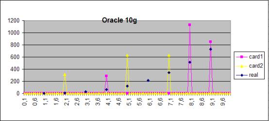
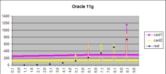
Figure1 The result of the estimation of the cardinality for the
statement
Select * from t_inc2 where x = :1 for values between 0 and 10. Two sets
of optimizer statistics are
considered (yellow and pink) based on the identical data with the default
sample size. The real cardinality is shown for comparison (blue).
This is of course good news. There seems to be a sort of anti-aliasing (http://en.wikipedia.org/wiki/Anti-aliasing)
carried out in Oracle CBO 11g.
Followup: Greg Rahn pointed out in a mail that the release I used (10.2.0.1) … read the full story
Jaromir D.B. Nemec
Created 29.11.2008
Last revision 6.1.2009
Jaromir D.B. Nemec is a freelancer specializing in data warehouse and
integration solutions. He can be reached under http://www.db-nemec.com