Flipping Execution Plan II
Greg Rahn pointed out in a mail that the release I used (10.2.0.1) in
the previous example is a rather old one.
This is of course true. I upgraded to 10.2.0.4 and realized that the example
doesn’t work; the plan doesn’t change (similar to the 11.0.6 behaviour). This
is caused by the fact that the variation of the cardinality (caused by random
sampling of the data to build the histogram) is much smaller than in 10.2.0.1.
So the execution plan in the new version doesn’t change.
In short: the cause of the problem is still there but the effect are
must smaller in higher releases.
It took me some time to find a more sensitive example that causes the
plan flip in 10.2.0.4 (and in 11g):
select *
from t_inc2
a where a.x = 8 and
5 < (select avg(val) from
t_inc_det b where b.y = a.y);
I added a detail table used in a correlated subquery. The CBO tends
for a lower number of rows of the main table (t_inc2) to hash join both tables
and then to aggregate and filter (i.e. subquery unnesting). For a higher number of rows CBO first aggregates the whole
detail table, performs the filter and then joins the result with the main
table. This behaviour is illustrated in Figure 1.
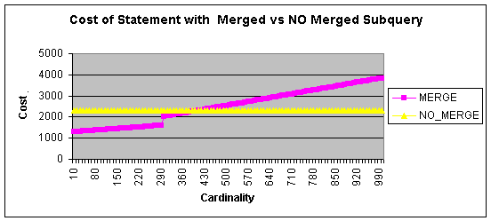
Figure 1 The cost of the merged and no merged plans
dependent of the cardinality of the predicate T_INC2.x = :1
In Figure 2 there is a graph of the CBO estimation of the result
cardinality for the predicate x = <value> for the table T_INC2. The graph
represents five states taken after re-collecting statistics with default sample
size. Details see above.
Figure 2
The result cardinality of the predicate T_INC2.x = :x for the interval [0..10]
in four different gathering of the table statistics
So the only “difficulty” to construct the flipping example is to choose
a constant value in the predicate x = <value> so that the resulting
cardinality lies both in the left and right side
of the graph in Figure 1.
Here is the update script to setup the
environment and the results of a run script in 10.2.0.4 and 11.1.0.6.
Via a grep of the spool file we can see
the changes of the execution plan.
$ grep 'HASH'
run_flip_v2.log
1
0 HASH JOIN (Cost=2445 Card=66
Bytes=8778)
4
3 HASH (GROUP BY) (Cost=2188 Card=50 Bytes=550)
2
1 HASH (GROUP BY) (Cost=1593
Card=1440 Bytes=169920)
3
2 HASH JOIN (Cost=1287
Card=28787 Bytes=3396866)
--- cut to save space
---
The first two lines correspond to the execution plan performing the
aggregation of the detail table in the first place and joining the filtered
result with the master table. Note that the estimated cardinality of the master
table is 582 (see the execution plan below). The last two lines in the grep result
represent the second option. The CBO first performs the join of the master and
detail tables and in a second step the aggregation ‘hash (group by)’ and
filter. Note that in this case the estimated cardinality of the master table
was only 288. See the full execution plan below.
Execution Plan –
Subquery Processing
----------------------------------------------------------
0
SELECT STATEMENT Optimizer=ALL_ROWS (Cost=2445 Card=66 Bytes
=8778)
1
0 HASH JOIN (Cost=2445 Card=66
Bytes=8778)
2
1 VIEW OF 'VW_SQ_1' (VIEW)
(Cost=2188 Card=50 Bytes=1300)
3
2 FILTER
4
3 HASH (GROUP BY)
(Cost=2188 Card=50 Bytes=550)
5
4 TABLE ACCESS (FULL)
OF 'T_INC_DET' (TABLE) (Cost=9
99 Card=100000 Bytes=1100000)
6
1 TABLE ACCESS (BY INDEX
ROWID) OF 'T_INC2' (TABLE) (Cost=
255 Card=582 Bytes=62274)
7
6 INDEX (RANGE SCAN) OF
'T_INC_IDX2' (INDEX) (Cost=6 Car
d=582)
Execution Plan –
Unnesting of the subquery
----------------------------------------------------------
0
SELECT STATEMENT Optimizer=ALL_ROWS (Cost=1593 Card=1440 Byt
es=169920)
1
0 FILTER
2
1 HASH (GROUP BY) (Cost=1593
Card=1440 Bytes=169920)
3
2 HASH JOIN (Cost=1287
Card=28787 Bytes=3396866)
4
3 TABLE ACCESS (BY INDEX
ROWID) OF 'T_INC2' (TABLE) (C
ost=128 Card=288 Bytes=30816)
5
4 INDEX (RANGE SCAN) OF
'T_INC_IDX2' (INDEX) (Cost=4
Card=288)
6
3 TABLE ACCESS (FULL) OF
'T_INC_DET' (TABLE) (Cost=999
Card=100000 Bytes=1100000)
Summary
I discussed this behaviour with Wolfgang Breitling (www.centrexcc.com) at UKOUG
Conference. His statement was fairly simple: “Don’t sample histogram!”. This
seams to me to be the best solution to the above problem, as
1) histogram should be defined on a column with skew data and
2) skew data may cause random results if sampled with inappropriate sample
size.
Jaromir D.B. Nemec
Last revision
6.1.2009